Ocean Surface Wave Spectrum Revisited — Part II: From Surface Displacement to the Ocean Wave Spectrum
The second part of the update to my (incomplete) review on spectral models for ocean waves
This is the second part of the update to my research note entitled Ocean Surface Wave Spectrum that I published on my ResearchGate. If you want to read the first part, click here.
From Ocean Surface Displacement to the Ocean Wave Spectrum
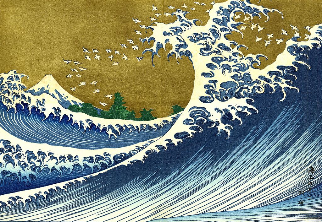
As described in Part I, the ocean surface can be described as the superimposition and interaction of individual waves, each one with a different history, stage of development, direction, generating and restoring forces, and time and length scales. A visualization of the interaction between ocean waves is shown in the diagram by Shearman
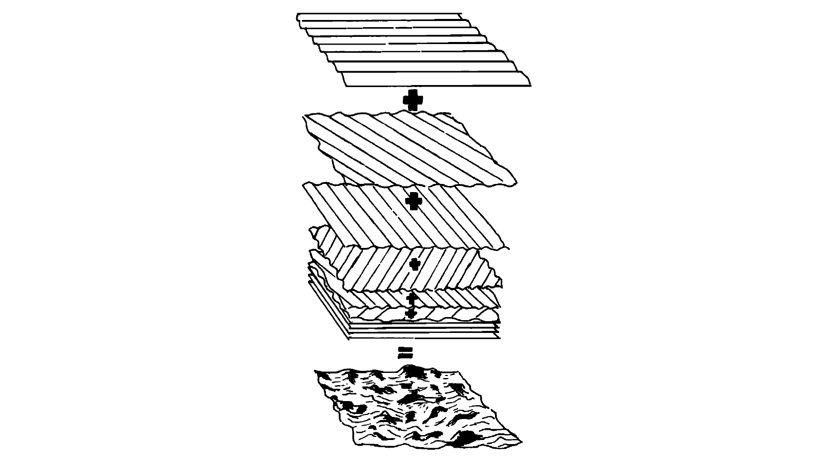
In theory, using the superposition of linear waves as presented by Feddersen
From the tools available to treat random surfaces, spectral analysis is the best suited to extract the energy, spatial and frequency characteristics of the ocean surface. In simple terms, the goal of the spectral analysis of the ocean surface is to mathematically “reverse” the process of wave superposition, following the diagram in the figure backwards to identify the energy and dominant direction for a given wavelength. This information is encapsulated in the power spectral density of the ocean waves, also known as the ocean wave spectrum, usually represented as a function of wave frequency or wavenumber. A detailed treatment of the spectral analysis of the ocean waves is presented by Massel
Directional Ocean Wave Spectrum
At any given point of the ocean surface, the vertical displacement caused by the ocean waves can be represented by a time-varying random process \(\zeta(\vec{\rho},t)\), where \(\vec{\rho} = (x,y) = \rho\angle\theta_r\) is the position of a point on the ocean surface. According to the Wiener-Khinchin theorem, the power spectral density of a wide-sense stationary random process can be defined as the Fourier transform of its autocorrelation function. If the surface displacement \(\zeta(\vec{\rho},t)\) is assumed to be a wide-sense stationary and ergodic process with mean \(E\left\{\zeta(\vec{\rho},t)\right\} = \overline{\zeta} = 0\), the autocorrelation of the ocean surface can be written as
where \(\vec{r}\) and \(\tau\) are the space and time lags for the autocorrelation, and the overbar indicates the conjugate of the function. Therefore, the wavenumber-frequency spectrum of the ocean surface can be defined as
where \(\vec{k} = (k_x,k_y) = (k\cos\theta,k\sin\theta)\) is the spatial frequency vector of a wave moving in the \(\theta\) direction with wave number \(k = \frac{2\pi}{\lambda}\). The wavenumber-frequency spectrum is the most complete spectral description of the ocean surface, as it has the advantage of being independent of the dispersion relation of the ocean waves. However, its practical use is not as common as the directional ocean wave spectrum, which provides a spectral description of the ocean surface using only the wave frequency (or wavenumber) and the wave direction for each frequency. As described by Donelan et al.
Since the ocean waves are dispersive with a known dispersion relation for specific cases, it is more common to approximate the ocean wave spectrum using the dispersion relation of the ocean waves, as it facilitates the integration in \eqref{eqn:Hatswtheta}. Assuming that the dispersion relations derived in Part I hold, the frequency-dependent directional ocean wave spectrum for deep-water waves can be approximated as
According to Donelan et al.
While it is common for studies in physical oceanography to express ocean wave spectrum models as a function of wave frequency, HF-radar scattering studies usually employ the wavenumber spectrum; this is especially true for works related to the radar cross-section of the ocean surface in the HF band. Similar to the \eqref{eqn:Swtheta}, the approximation of the wavenumber-dependent directional ocean wave spectrum for deep-water waves can be defined as follows:
As described by Massel
Therefore, even if a model is presented as a frequency-dependent spectrum, the wavenumber-dependent spectrum can be obtained using \eqref{eqn:SktoSw}. Since the spectral models for the ocean surface are usually described as a function of frequency, and knowing that the wavenumber spectrum can be obtained from the frequency spectrum, the derivations from this point onward in these notes are going to focus on the frequency-dependent ocean wave spectrum.
Non-Directional Ocean Wave Spectrum and Directional Factor
Due to the complexity of wave-wave and wind-wave interactions, obtaining accurate directional information from the ocean surface is a complicated technical problem. Therefore, the majority of the experiments designed to obtain surface displacement information focuses on obtaining the frequency spectrum of the ocean surface, with the directional information obtained through empirical parameters and mathematical models of the directional spreading of ocean waves
The functions are defined as follows:
- \(\hat{S}(\omega)\): a frequency spectrum, containing the energy information for each wave frequency on the ocean surface;
- \(D(\theta,\omega)\) : a directional factor, which relates wave frequencies and their dominant wave directions. The parameters for the directional factor are:
- \(\theta\): direction of observation for the wave with frequency equal to \(\omega\);
- \(\omega\): frequency of the wave being observed;
- \(p_1,p_2,\cdots\): empirical parameters used to describe the directional spreading of the ocean waves. For simplicity, these parameters will be omitted unless required for the analysis.
From the directional spectra, the frequency spectrum can be obtained by further integrating the wavenumber-frequency spectrum in \eqref{eqn:Swtheta} over \(\theta\):
Based on the definition of the frequency spectrum shown in \eqref{eqn:Sw}, the directional factor is then defined such that
$$ \int\limits_{-\pi}^{\pi} D(\theta,\omega)\mathrm{d}\theta = 1,\ \forall \omega. $$
A similar definition can be obtained for the approximation of the ocean wave spectrum for deep-water waves. The frequency spectrum in this case can be defined as
Next Steps
Now that the directional spectrum has been mathematically defined, we will dive into the frequency spectrum more specifically. The next installment of this series will explore the similarity laws for the frequency spectrum, which will help us define the important variables to define a model for the ocean surface.
If you are interested in the directional factors, don’t worry. The different models for the directional factor will be explored in future installments of this series.