Ocean Surface Wave Spectrum Revisited — Part I: Wave Generation and Classification

An update to my (incomplete) review on spectral models for ocean waves

So, I’ll start my blog with something that I wanted to do for a long time: write a correction/expansion to the research note entitled Ocean Surface Wave Spectrum that I published on my ResearchGate profile in 2015. But first, I’ll give some context on how these notes came to be.

When I started my Masters at MUN, my supervisor listed four courses as my suggested coursework: Applied Remote Sensing, Digital Signal Processing, Antenna Theory and Physical Oceanography. As the Sesame Street song goes, “one of these things is not like the others.” Coming from an undergrad in Electrical Engineering, taking a course in Physical Oceanography seemed like an odd choice, but my supervisor convinced me by saying “if you are going to study remote sensing of the ocean, you have to at least know how your target works.” To my surprise, it turned out that I liked that course a lot. Part was Prof. Munroe way of teaching it, and another part was that I found the subject actually very interesting.

One of the last evaluations of the Physical Oceanography course was a small tutorial, in which we would have the time of one class to explain one topic related to the course that we wanted to cover. So, I chose spectral models for ocean waves, since my Masters work would involve the extraction of the wave spectral information from received radar data. For the tutorial, we would have to write some lecture notes, which I did in the form of the “Ocean Surface Wave Spectrum” research note. I liked these notes so much that I published them on ResearchGate before I got the corrections form Prof. Munroe; that turned out to be a mistake. There were some important corrections that didn’t go into the published version of the note, which now has almost 8,000 reads as of writing this post (!!), and two citations (!!!). Also, after going deeper in the concepts of related to ocean wave spectral models over the years, there are some topics in the notes that I think deserve more attention. So, while I didn’t update the note itself on ResearchGate, many of the concepts explained in the lecture note were expanded in my master thesis, which are one of the sources of the content presented here.

So, without further ado, here are the updated notes.

Introduction

As explained by Massel , ocean and atmosphere, by their nature, form a thermodynamic coupled system, continuously exchanging heat, mass and momentum on their interface. This means that any forcing that is imposed from one fluid to the other generates a response that will change the interfacial conditions of the system, modifying the boundary between the fluids. Considering the ocean-atmosphere system, waves are the responses from the ocean surface due to external forces.

One of the main features of the ocean surface is its inherent randomness, caused by a response over time and space to a variety of external forces at different time and length scales, as well as different energy contents, directions and natures (e.g. wind waves vs coriolis waves). Waves generated by distant storms mix with waves generated at the observed region, all of them mixing with other kinds of waves, such as planetary waves. With this multiplicity of sources, it is not possible to deal with the sea with a deterministic approach. So, instead of trying to identify the sources and behaviours of each single contributor to an observed ocean wave, treating the ocean as a random surface and using tools of stochastic analysis might provide a better insight on the ocean behaviour, energy content, and how it can be modelled over time and space.

The periodicity of the ocean surface also suggests the use of frequency domain techniques, of which spectral analysis is the most widely used. Stochastic spectral analysis can deal with the distribution of energy in different frequencies and directions, which makes it suitable for ocean surface mapping. The directional ocean wave spectrum, is the most comprehensive measurement in the study of the upper ocean, and other measurements such as significant wave height, peak wave period, and dominant wave direction can be determined from it.

But before examining the ocean wave spectrum itself, it is important to understand how the different types of waves can be classified.

Ocean Wave Classification

One of the painting in *Hatō zu* by Konen Uehara

According to Kinsman , there are several ways to classify ocean waves. Here we are going to present classifications based on the dispersion relation, other physical characteristics, and place of origin of ocean waves. It should be noted that all three classifications can, and usually do, coexist in the analysis of ocean waves; for example, the same wave can be classified as swell (place of origin classification), and a deep-water (dispersion relation classification) surface gravity wave (dispersion relation/wave period classification). Some are mutually exclusive due to physical characteristics; for example, a capillary wave (dispersion relation/wave period classification) cannot be classified as swell (place of origin classification), as the energy of capillary waves would not allow travel outside of the original ocean patch to be classified as swell. These exclusive cases become self-evident as the classifications are understood.

Classifications Arising from the Dispersion Relation

Considering the linear theory of ocean waves as presented, for example, by Stewart , some wave classifications can be derived directly from the dispersion relation of the ocean waves, which establishes a relationship between angular frequency and wavelength of the waves. As described, for example, by Phillips , the dispersion relation of ocean waves, discarding any the effects of viscosity or Coriolis forces, can be written as

\begin{equation} \label{eqn:disprel_full} \omega^2 = gK\left(1+\gamma \frac{K^2}{g}\right)\tanh(Kh), \end{equation} where $\omega$ is the angular frequency of the ocean wave, $g$ is the acceleration due to gravity, $K$ is the wavenumber of the ocean wave, defined as

$$K=\frac{2\pi}{\lambda},$$

with $\lambda$ being the ocean wavelength, $\gamma$ is the ratio between the surface tension and water density, and $ h$ is the depth of the ocean.

Considering first the terms in parenthesis in \eqref{eqn:disprel_full}, two classes of waves can be observed:

At wave-numbers $ K<\sqrt{\frac{g}{\gamma}}$, the restoring force for the ocean wave is predominantly gravitational. These waves are known as gravitational, or gravity waves.
For waves with $ K>\sqrt{\frac{g}{\gamma}}$ the restoring force is primarily surface tension, also known as capillarity. These waves are known as capillary waves.

Another classification can be found by analyzing the hyperbolic tangent in \eqref{eqn:disprel_full}. From its argument, waves can be classified according to the ratio between depth and wavenumber:

When $Kh \gg 1$, or $h \gg \lambda$, $\tanh(Kh)\approx 1$, making the dispersion relation of these waves completely independent of water depth. These waves are called deep water waves.
When $Kh \ll 1$, or $h \ll \lambda$, $\tanh(Kh) \approx Kh$, making the dispersion relation directly proportional to the water depth. These waves are classified as shallow water waves.
If neither of these conditions is satisfied, the wave is said to be of intermediate depth or are called intermediate water waves.

Classification Based on Wave Period

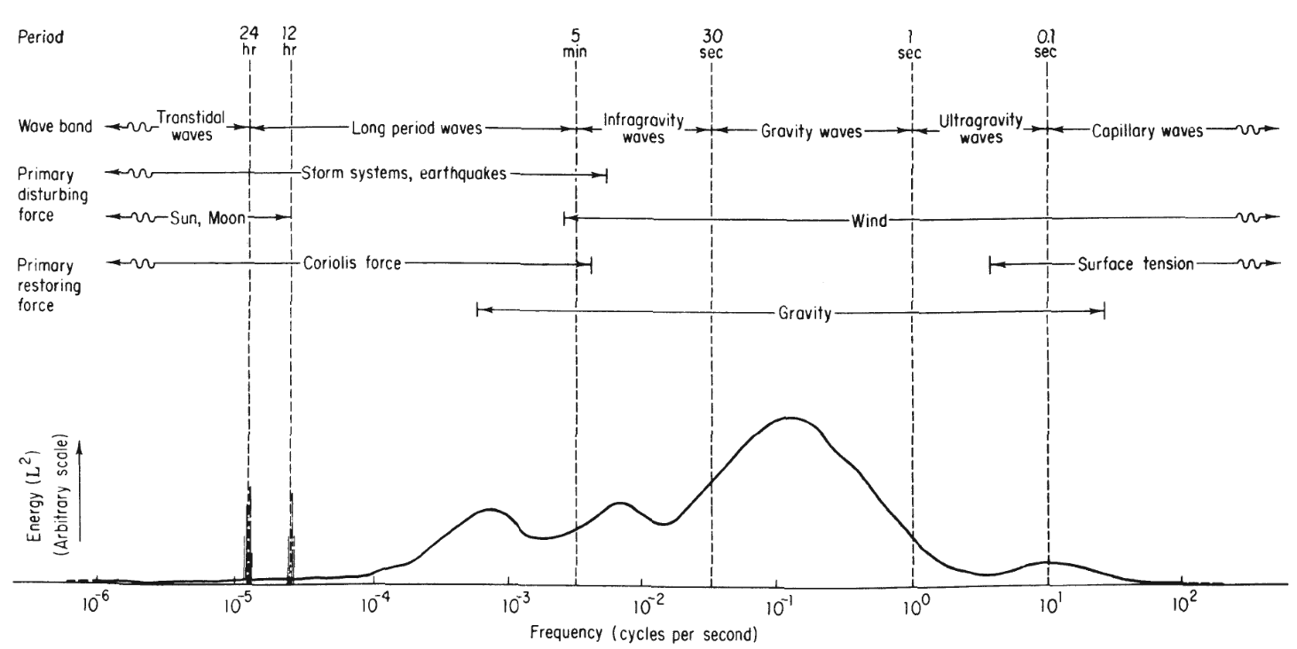
Another classification method, presented by Munk and expanded by Kinsman , classifies waves according to their periods, or, reciprocally, their frequencies, as shown in the figure above. In the classification presented by Kinsman , there are six types of waves, based on their wave periods, here denoted as $T$. Munk also established which are the events or forces that generate these waves, as shown below:

Classification of ocean waves according to wave frequency, with relative energy, generating disturbances and restoring forces for each type of wave. Image published by Kinsman

Capillary waves: Waves with period $T < 0.1\text{ s}$. These waves are generated by the wind and restored by surface tension, also known as capillarity. As the period approaches $0.1\text{ s}$, gravity starts to contribute to the restoration of capillary waves.
Ultra-gravity waves: Waves with period $0.1\text{ s} \leq T < 1\text{ s}$. These waves are generated by the wind and restored by a combination of gravitational effects and surface tension.
Gravity waves: Waves with period $1\text{ s} \leq T < 30\text{ s}$. These waves are generated by the wind and restored by gravity.
Infra-gravity waves: Waves with period $30\text{ s} \leq T < 5\text{ min.}$. According to Munk , these waves are generated as a result of the development of wind and ordinary gravity waves, so, the primary generating force is the wind. The primary restoring force of these waves is gravity.
Long-period waves: Waves with period $5\text{ min.} \leq T < 24\text{ h}$. According to Munk , this class can be divided in two groups:
- Ordinary long-period waves: Waves with periods between $5\text{ min.} \leq T < 12\text{ h}$. These waves are generated by storm systems and earthquakes and restored by Coriolis forces.
- Tidal waves: Waves with period $12\text{ h} \leq T < 24\text{ s}$. These waves are generated by lunar and solar gravitational cycles, as well as storm systems and earthquakes. The primary restoring force of these waves are Coriolis forces.
Trans-tidal waves: Waves with period $T \geq 24\text{ h}$. These waves are generated by lunar and solar gravitational cycles, as well as storm systems and earthquakes. The primary restoring force of these waves are Coriolis forces.

Classification Based on the Direction of Pressure and Density Gradients

As described, for example, by Cushmain-Roisin and Beckers , the ocean water is a nearly incompressible fluid, with density changes dominated by salinity and temperature. Since both the salinity and temperature of the ocean changes with depth, the density of the ocean also changes with depth, making the ocean a stratified fluid. This produces a density gradient which, due to gravity, tends to be vertical when undisturbed, stacking with the lower densities at the top and higher at the bottom, creating an interface between fluids of different densities, similar to the one present at the surface. The main difference between these internal layers and the surface layer is that the fluids in the first case have comparable density, while the difference in density in the second case is much larger.

Evidently, differences in water depth will cause a vertical pressure gradient, so, the water density can be mapped as dependent on pressure. However, changes in salinity and water temperature can cause a change in the direction of the density gradient, breaking its dependence with water depth and, consequently with the pressure gradient. This creates two classes of waves, as described by Sutherland :

Barotropic waves: Waves in which the density and pressure gradients are aligned. This is the case for all surface waves, since the compressibility of the air at the upper layer enforces the direction of the density gradient. This class also includes waves caused by Coriolis forces, such as Kelvin waves, Poincaré waves, topographic waves, and planetary or Rossby waves .
Baroclinic waves: Waves in which the density and pressure gradients are misaligned. This happens at internal waves, which are explained in detail by Sutherland .

Classifications Arising from Place of Origin

In his classification of ocean waves, Kinsman further divides the gravity waves in two different states, considering whether the waves have been generated at the point in question. In other words, Kinsman classifies these waves in terms of their place of origin. The place of origin classification of gravity waves is divided in two groups:

Sea: Waves that have been generated by the local wind. These are waves with shorter periods, with a large variation of steepness and direction over time and space.
Swell: Waves that have not been generated by the local winds, and have escaped their original ocean patches. These waves are longer in period, and tend to be more uniform over time and space.

According to Kinsman , a good rule of thumb to separate sea and swell is the following:

$$ \begin{cases} T \leq 10\text{ s}: & \text{Sea}\\ T > 10\text{ s}: & \text{Swell.} \end{cases} $$

However, in practice, this distinction is not as clear as the rule-of-thumb suggests. Depending on the development state of the local waves, swell and sea can appear mixed in the ocean wave spectrum. Furthermore, the correlation between the direction of propagation of the waves in the observed patch and the local winds is also important to determine the place of origin of the ocean wave. For that matter, methods to identify sea and swell in the ocean wave spectrum have been developed over the years. Some examples are the ones presented by Wang and Hwang , Ewans et al. , and Hwang, Ocampo-Torres, and García-Nava .

The classification of sea and swell is an important part of the study of ocean waves, especially on the remote sensing of the ocean surface. For example, if the objective is to study the locally-generated ocean waves and its relation to the local winds, the presence of swell might distort the perception of the ocean surface; on the other hand, if the objective is to study the propagation of waves generated by a particular storm, the presence of local waves can complicate the observations.

Wind Wave Generation and Development

Kojima Zu, painting by an unknown artist between 1890 and 1920

At this point, we should recognize that the object of study of these notes are what Kinsman classifies as wind waves. As the name suggests, these waves are the result of atmospheric forces over the ocean surface. Observing the classification provided by Kinsman , wind-generated waves can span from small capillary waves to large gravity waves caused by storm systems. Before moving to an analysis of the wave spectrum, it is important to understand the life cycle of an ocean wave, how the are generated and how they develop.

According to Phillips and Massel , the development of a more widely accepted wind wave generation theory came in the 1950’s, especially after the publication of two papers, one by Phillips himself , and another by Miles , both published in 1957 in the Journal of Fluid Mechanics. Even though the research behind these papers was developed independently, the two proposed mechanisms are in fact complementary and are also referred to as the Miles-Phillips mechanism.

The Miles-Phillips mechanism can be described in a thought experiment, in which each part of the theory can be understood. At first, a flat air-sea interface, without any perturbation from each of the fluids is considered. If pressure variations are introduced into the atmosphere and transmitted to the air-sea interface, these pressure variations will resonate on the interface itself, due to the fact that this is a coupled thermodynamic system. These pressure variations cause small ripples in the ocean surface as a response to the initial pressure variations. This process is known as the Phillips’ resonance mechanism.

Phillips’ theory can successfully explain the initial growth of the waves, but cannot describe their further growth properly. The waves described by Phillips’ theory are most likely capillary waves, and would propagate and dissipate through the ocean surface using its surface tension if these pressure variations were to cease. However, if a parallel shear flow is applied over the rippled surface, energy will be transferred from the wind to these small ripples at a much higher rate than Phillips’ theory would predict. The waves affected by this parallel shear flow would rapidly grow in size and speed, which would change their restoring forces from surface tension to gravity. The process responsible for wave growth due to a shear wind flow is known as Miles’ shear flow mechanism.

These waves, however, cannot grow indefinitely. As described by Massel , when waves meet some criteria, such as their wave height to wavelength ratio reaching 1/7 or their particle velocity at the crest being equal to the wave phase speed, they start to destabilize, becoming what are known as breaking waves. The detailed theory on how and when the waves break is presented by Massel .

Next Steps

Now that the wave generation process and the different classes have been established, the process of defining a spectral model for the ocean surface can be explained in more detail.